Down the (Transmission) Line:

Guiding Waves Integrally

Daniel M. Dobkin
revised December 2012

A Lonely Wire: Why Waves Won't Go

How do we get a wave to go down a wire?

Let's try using a single isolated wire of constant cross-section, with radius much smaller than a wavelength, so that we can assume the current is constant around the wire. If a signal is propagating on the wire, there are currents flowing on the surface and charge accumulates if the current is not constant along the length of the wire. The problem is shown below (taking charge carriers as positive for convenience if not physicality):



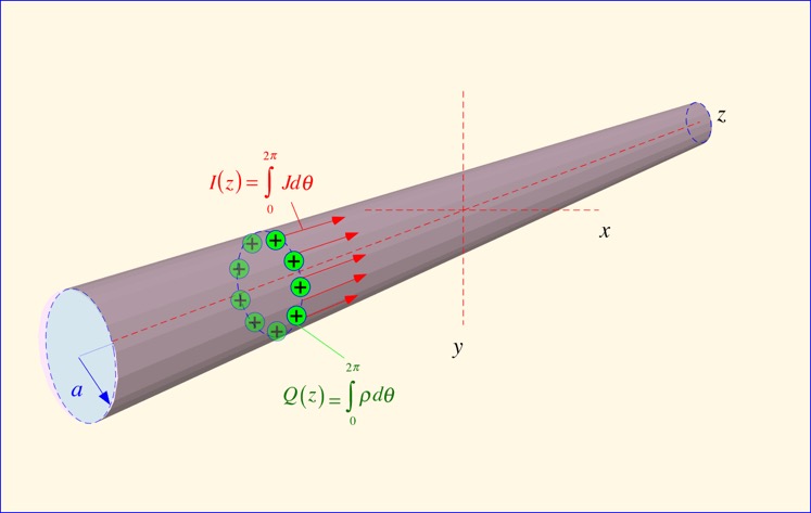
Let us assume that the current has the form of a traveling wave; with implied harmonic time dependence e^iωt we can write:



Now, charge and current are not independent, since charge is conserved: a change in the current with space results in an accumulation of charge over time, that is:



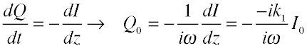
where the last equation is obtained recalling that the derivative of an exponential just brings down a constant factor when the argument is linear. Recall that the velocity of a wave is the ratio of the wavenumber k and the angular frequency ω, enabling us to re-express this as:


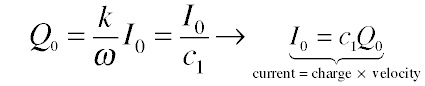
That is, the current in the traveling wave is composed of charge traveling at the same velocity the wave propagates at.

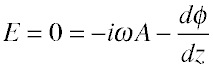
In order to go further, we need to ask whether this solution makes sense. How do we do it? As we noted previously, for reasonably high frequencies all the current flows on the surface of the wire. Therefore the electric field must be zero inside the wire, where no current is flowing. But we know how to find the electric field: we perform a delayed integral over the current to get the vector potential, and integrate over the charges to get the scalar potential. The sum of the time derivative of A (which has only a z component) and the gradient of φ is the negative of the electric field. (See Useful Tools.)



In this case, we have not assumed that the wire length is small compared to a wavelength -- in fact, the reverse -- so we must account for the delay, or equivalently the phase shift, between the place where the charge or current is and the location at which we measure the potential. Substituting our assumed form for the current and the charge derived above, and choosing to measure the potential at z = 0, we find the source integrals:



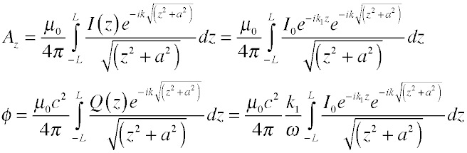
where L is the half-length of the wire. Notice that the integral is of the same form in both cases. As long as it is finite we can ignore the details and write the following equation for the electric field in the center of the wire at z=0:



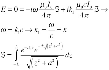
That is, the phase velocity of the wave along the wire must be equal to the velocity of light in vacuum.

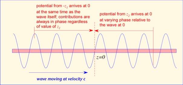
Now let's take a closer look at the integral. It is composed of two rather different halves: one extending in the same direction as the wave is traveling (future-ward, if you will) and one in the direction from which the wave has come (past-ward). In the pastward direction, z<0 and the two exponential terms essentially cancel except for small values of z, and the integral becomes of the form of an integral of 1/z. In the futureward direction, the two exponentials add and thus phase varies rapidly with increasing distance; as a result, the futureward integral is dominated by the contribution of nearby currents or charges.




Mathematically speaking:



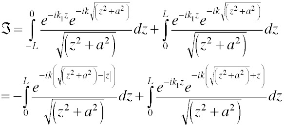
The right-hand integral will converge to a finite value if the distance to the right end of the line is very long, and the value will be independent of the actual length. However, the left-hand integral is essentially just ln(L/a) for L>>a, with a modest phase factor. Unfortunately, the logarithm grows arbitrarily (albeit rather slowly) as the length grows: the value of the integral is not constant with position for a long wire. While a traveling-wave solution is possible, the resulting potentials are dependent on the absolute length of the wire. We usually like to think of a transmission line as a device that directs a signal whose properties vary only in phase with position along the line; a single wire won't do it for us.

Two Wires: Currents in Opposition

To solve the problem of divergence of the source integrals, we can introduce a second wire, spaced some distance (small compared to a wavelength) from the first. If the currents on the second wire are equal in magnitude and opposite in direction from those on the first, it is reasonable to guess that the potential arising from distant currents on the first wire will be cancelled by that from opposing currents on the second wire, since for large values of z, the separation between the wires will have little effect on the distance. Only the current and charge near the point of observation, where the distance between the wires is important, will contribute to the local potentials. So here's a twin-wire transmission line, with the separation between lines δ presumed large compared to the wire radius a but still small compared to the wavelength.



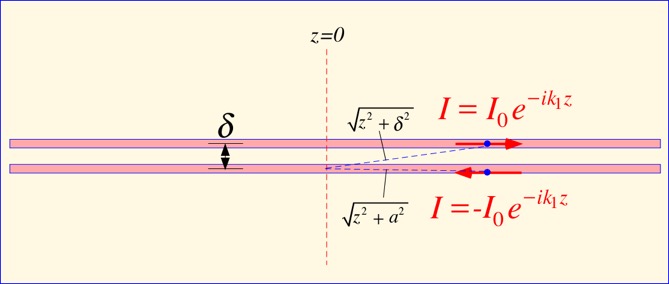
The source integrals for the potential at the center of one of the wires become:




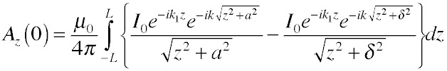
(where we have assumed the radius is small compared to the separation, so we can neglect the radius of the more distant wire). Now, the key observation to make here is that the two terms in each integral become essentially equal when |z| >> a and δ. So, unlike the case of a single wire, as long as the wires are reasonably long compared to their radius and separation, we can reasonably expect the potentials to be independent of the wire length, and thus of position along the wires (except for the phase). It is sensible to treat solutions in this case as traveling waves that move along the wires without changing their properties.

Furthermore, if both radius and separation are small compared to a wavelength, the phase terms kz are very small and can the neglected in the region where the contribution to the integral is significant: the exponentials simply become = 1, and the integrals turn into very familiar forms. We can integrate out to some reasonable multiple of the separation in each direction and show that the result is essentially independent of the choice of multiplier:



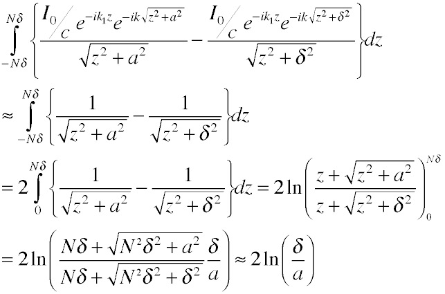
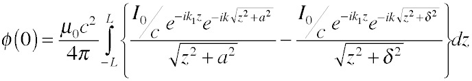
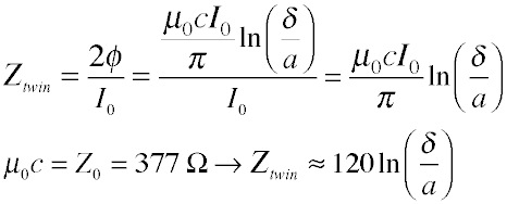
This means that the potentials are independent if position along the wire (save for variations in phase), as is desired for a transmission line. With the integral in hand we can find the characteristics of the transmission line. For example, the impedance of the line, the ratio of the voltage to the current, is the difference between the scalar potential on one wire and the other at the same position z, divided by the magnitude of the current. Since by symmetry the potential is zero between the wires, this is just twice the potential on one wire, divided by the current. Substituting for the value of the integral in the source equation, and recalling that the product of permeability and the velocity of light is the impedance of free space, Z₀, we get:



We can also use this expression for a coaxial cable if we realize that the potential outside the shield must be 0, so the potential to put into the expression is just the potential at a. Thus the impedance is roughly half that of a twin wire transmission line for the same dimensions:



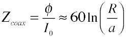
where R is the radius of the outer conductor.